Logistic regression deals with dependent variable, which is either dichotomous (binary logistic regression) or categorical without any inherent order (multinominal logistic regression). More common is binary logistic regression because it encompasses diversity of situation with common feature, such as the absence or presence of some predicted parameter in particular observation, and this type of regression will be discussed below.
When dependent variable is measured in dichotomous scale (0/1), for study of relationship between this variable and one or more predictor variables it is impractical to use linear regression. In linear regression dependent variable may take values greater than 1 or lower than 0, however when values fall in ranges between 0 and 1 logistic regression is used. The logistic regression belongs to generalized linear models with specific feature that it links the range of real numbers to the 0-1 range.
In contrast to linear regression, logistic regression does not assume a linear relationship between dependent and predictor variables, the predictor variables are not required to be interval or normally distributed, and the variances within each group are not required to be equal. It requires another condition – categories of dependent variable must be mutually exclusive and exhaustive, and each case can be only the member of one group. Likewise, there is a recommendation that amount of cases should be at least 50 because for better estimation larger samples are needed than for linear regression.
During logistic regression analysis, similar to linear regression, coefficients for predictor variables are estimated with producing of regression equation. Final purpose of this procedure is to estimate probability (p) of predicted event.
Logistic regression equation has the following view:
Logit(p): = a + b1x1 + b2x2…,
where a – the constant of equation (intercept), b1, b2... – coefficients of the predictor variables, x1, x2… - predictor variables, Logit(p) is the logarithm (to base e) of the odds ratio or likelihood ratio that the dependent variable is 1:
Logit (p) = ln[p/(1 – p)].
If the regression equation is designated as “X”, than the probability of event is calculated by the following formula:
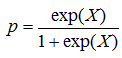 ,
,
where exp is the base of natural logarithms (approximately 2.72).
Logistic regression in SPSS
We continue discussing the example on patients with sterile and infectious forms of acute pancreatitis (see Discriminant analysis, Example 8). By the discriminant analysis we predicted in which group the most probably will fall the patient. Logistic regression also predicts membership of patient and answers the question about probability to belong to either of groups. There is an obvious difference whether the patient has infectious form of diseases with probability of 55% or 99%.
To start logistic regression analysis in SPSS:
1. Click the Analyze menu, point to Regression and select Binary Logistic… :

Logistic Regression dialog box opens:

2. Select the dependent variable (“Infection”), click the transfer arrow button  . The selected variable is moved to the Dependent: list box.
3. Select the predictor variables (covariates) (“ELR” and “SAPS III”), click the transfer arrow button in the section Block 1 of 1, the variables are moved to the Covariates: list box.
4. Regression method we may keep chosen by default “Entry”, other way we may choose any of forward or backward methods:

5. If we have any categorical variable/s we should click the Categorical… button and then in the dialog box Logistic Regression: Define Categorical Variables. select these variables and move to the Categorical Covariates: list box:

However, in our example there are no categorical variables.
6. Click the Options… button, the Logistic Regression: Options dialog box opens:

7. Select Classification plots, Hosmer-Lemeshow goodness-of-fit and Casewise listing of residuals check boxes. Other options leave selected by default. Click the Continue button. This returns you to the Logistic Regression dialog box.
8. To perform later ROC-analysis it is useful to save predicted probabilities. Click the Save… button. The Logistic regression: Save dialog box opens:

9. Select Probabilities check box. Click the Continue button and then in the main dialog box the OK button. The Output Viewer window opens with results of logistic regression analysis.
Apart from general information, such as the table Case Processing Summary which contains number of included and missed cases and the table Dependent Variable Encoding with codes for dependent variable, the Output Viewer window contains two blocks of tables – Block 0 and Block 1.
The Block 0 contains information about initial model which has only constant before including any variables:

The purpose of further analysis is to assess, whether the model with variables is better than initial model. This block contains three tables - Classification Table, Variables in the Equation and Variables not in the Equation. The first table shows the probability of correct classification of the observation if we do it simply by chance, in our example it is 69.1%. That is, if without any modeling we define that our patient has infectious form, in 69.1% of cases we will take correct decision. Next two tables show that no predictors were included in the model on this stage. However, as it is seen from the third table, including of the variable “SAPS III” will significantly improve the initial model. If both variables were not significant, then termination of analysis would be rational on this point.
The Block 1 contains statistics for the built model itself. It has six tables and a chart. The table Omnibus Tests of Model Coefficients has the information about model fit:

The Model Shi Square indicates overall model significance, it is derived from the likelihood of observing the actual data under the assumption that the model which has been fitted is accurate. Here null hypothesis states that fitting of initial model (present in the block 0) is good, and alternative hypothesis states that it is not good and predictors have significant effect on the dependent variable. If the Chi-square test is statistically significant, then we can reject null hypothesis, and it means that model built in this step is better. This table has one step because we used entry model, but when forward or backward models are chosen, then all steps necessary to improve the predictive power of the model are demonstrated.
For the linear regression the most important parameter which estimates its characteristics is the coefficient of determination R2. In the logistic regression there are no close analogous statistics for the coefficient of determination, but some similar approximations which have similar properties to the true R-squared statistics were designed (so-called pseudo R-squared statistics) and are present in the table Model Summary, such as Cox and Snell R square and Nagelkerke R square. Maximum of the Cox and Snell R square coefficient is usually less than 1.0 making it difficult to interpret. The Nagelkerke R square coefficient is changed in ranges from 0 to 1 and is more reliable, in our example it shows that only 24.3% of total variance is explained by the model. -2 Log Likelihood (-2LL) is used to assess the differences between -2LL for the null hypothesis model (initial with including only constant) and -2LL for the best fitting model. This parameter is important in stepwise regression: the variables chosen by the stepwise method should all have significant changes in -2LL.
The Hosmer and Lemeshow test is an alternative to the model Chi square. Principle of this test is that all observations are divided into 10 groups based on the calculated probability: first group includes observations with probabilities from 0 to 0.1, second – from 0.1 to 0.2, etc. Then each group is divided into two subgroups, where observations were predicted correctly and those where prediction was wrong. This is described in the Contingency table for Hosmer and Lemeshow test:

Expected frequencies are obtained from the model. In order to test the fit of the model, the probability is calculated from the chi-square distribution with 8 degrees of freedom. Null hypothesis here states that there are no differences between observed and model predicted values. If the test is not significant, it means that we cannot reject the null hypothesis and our model is good. This we see at the table with Hosmer and Leneshow Test: p = 0.765, that is our model is better than guessing by chance.
The Classification Tables contain information on proportion of cases classified correctly. From this table we see that overall accuracy is rather good: 72.1% of cases were classified correctly, but among sterile form accuracy was only 28.6%, so there are too many false-positive results.
Block 1 also contains the table Variables in the Equation. It has several important elements which give information about importance of each predictor in the equation. “B” value is used for the model equation; S.E. represents its standard error:

Therefore, our model can be written as:
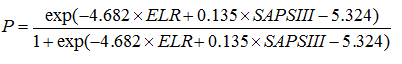
The Wald statistics and significance level is used for assessment of importance of each predictor in the model. Wald statistics for ELR variable is non-significant, therefore, it may be excluded from the model, and if we used stepwise regression, it would be automatically done. Exp(B) is useful in interpretation of B coefficients toward our data. It represents the ratio-change in the odds of the predicted event for a one-unit change in the predictor. That is, odds to have infectious form of the disease in a patient with 20 points by SAPS III score are 1.144 times the odds of a patient with 19 points if to assume that all other things are equal.
In terms of probability it is calculated in the following way:
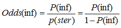 ,
,
where P(inf) is a probability to have infectious form in a particular patient.
If the patient has the probability to have infectious form of the disease 0.5, then the odds are: 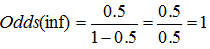 .
.
The odds of an infectious form for person who has SAPS III value 1 points higher are 1*1.144 = 1.144, and the probability to have infectious form is:
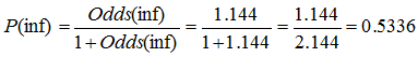 , therefore, the corresponding probability of having infectious form increases to 0.5336 from 0.5 which was in the first patient.
Another example: if the first patient has probability of infectious form 0.9, then the odds are:
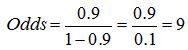 . The odds of the second patient with value of SAPSS III 1 point higher are 9*1.144 = 10.296.
Probability to have infectious form in the second patients will be:
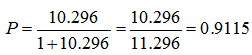 .
.
Notice that relative changes in probability to have infectious form in first set of patients (with initial probability of 0.5) was changed more (from 0.5 to 0.53) than in the second set of patients (from 0.9 to 0.91). In general, changes of probability are greater when they are near 0.5, and smaller when they are closer to 0 or 1.
The chart Observed Groups and Predicted Probabilities of the Block 1 makes it possible to assess visually classification of cases by the model:

When classification is done well the cases “0” are grouped at the left side and cases “1” at the right side with overall U-shaped picture. If distribution of cases is close to normal then classification is very poor and too many predictors are located near cut-off point. From our classification plot we can see that positive cases (“1s”) are in general classified better and there are many cases “0” near cut-off between 0.5 and 0.6 points.
The last table from logistic regression results contains description of poorly classified cases which require further greater attention. Outliers should be removed because they may significantly change results and then model should be built and assessed without outliers. There is a recommendation not to retain outliers if their standardized residuals are more than 2.58 (“ZResid” column):

During reporting the results of logistic regression, not only the equation itself should be written, but also values of Chi-square, degrees of freedom and p, Nagelkerke’s R, accuracy of model, Wald statistics with correspondent p and Exp(B) value because all these parameters give information about characteristics of the model.