The necessity of classification becomes obvious when dataset is too big and diverse to be analyzed only intuitively. Classification makes it possible to create subgroups of data which are more manageable and easier in interpretation from ‘formless mountain’ dataset. Classification methods belong to two principal categories. The first category is when we do not have any idea about how many groups can be built from our dataset, or our idea is only preliminary and we do not know which observation falls to which future group. In such cases cluster analysis is used, which helps to determine optimal number of groups and separate the objects between these groups. In another methods we already have an idea about number of groups, general properties of each group and even have information about membership of every our case; then this information is used for classification of future cases. Such methods include discriminant analysis and classification trees. The difference between these two methods is in nature of predictor (classifying) variables: in discriminant analysis predictor variables are only continuous, while in classification trees there are no restrictions in type of predicting variable.
The purpose of cluster analysis is to classify cases by minimizing differences within group and maximizing differences between groups, which are initially unknown. A term ‘cluster’ is used to describe the group of relatively homogenous cases or observations.
While in two-way and hierarchical clustering prior to performing classification the researcher does not have any idea about number of future groups at all, in k-means clustering number of groups is specified by researchers and then classification of cases is performed accordingly to these number of groups, providing maximally possible differences between clusters.
The most commonly used is squared Euclidian distance, which is an extension of Pythagora’s theorem. It gives geometric distance between two points in multi-dimensional space. Squared distance is used more commonly than simple Euclidian distance in order to give higher weight and express differences between objects which lie further apart. Both simple and squared Euclidian distances are usually calculated from raw data rather than from standardized ones.
Simple Euclidian distance: , where d – distance between object x and y, xi and yi – two objects.
Squared Euclidian distance: .
Pearson correlation is a product-moment correlation between two vectors of values.
Cosine distance is a cosine of vectors of variables: .
Block (city-block, or Manhattan) distance is the average difference across dimensions: . The effect of outliers is dampened here because distance is not squared. Such name was derived from the Manhattan district due to fact that in most American cities it is often not possible to go directly between two points, and a route which follows the regular grid of roads is used to calculate final destination.
Chebychev distance takes into account the absolute maximal distance between two objects among all dimensions; it also defines two objects as different if there is difference in at least one dimension: .
Minkowski distance is the generalized distance function which represents pth root of the sum of the absolute differences to the pth power between the values for the items: , when p = 1, Minkowsky distance is block distance, when p = 2, Minkowski distance is Euclidian distance.
Customized distance is even more generalized distance than previous one, it represents rth root of the sum of the absolute differences to the pth power between the values for the items: .
Clustering algorithms
Clustering algorithms differ in the way how distance between two clusters is defined. In SPSS present seven clustering algorithms: between-groups linkage (default procedure), within-group linkage, nearest neighbour, furthest neighbour, centroid clustering, median clustering and Ward’s method.
In the between-group linkage(average) method the distance between two clusters is calculated as the average of all distances between objects belonging to the two clusters.
In the within-group linkage method the distance between two clusters is measured as the average of all possible distances between objects within a single new cluster determined by combining together original clusters:
In the nearest neighbour (single linkage) method the distance between two clusters is measured as the minimum distance among all possible distances between object belonging to the two clusters.
In the furthest neighbour (complete distance) method, oppositely, distance between two clusters is measured as the maximum distance among all possible distances between objects belonging to the two clusters:
Centroid clustering algorithm includes determining centroids (means for each cluster) and then measuring distances between these centroids.
Median clustering method includes determining median for objects belonging to each cluster and then measuring distances between these medians. Similar to centroid method, but instead of mean median is used.
Ward’s method differs from other clustering algorithms because it uses analysis of variance approach in evaluation the distances between clusters. This method attempts to minimize the sum of squares of any two clusters that can be formed at each step. In other words, it minimizes within-cluster variation during grouping of objects into clusters:
Application of cluster analysis in biomedical studies
In biology and medicine, cluster analysis is mainly used for a study of genetic sequences in microorganisms, for example, for comparison of bacteria by restriction fragment length polymorphism. But sometimes cluster analysis is also used for different other purposes, for example, classification of bacterial aquatic environments (Bell and Albright, 1982), classification of isoenzyme profiles in Candida spp. (Lehmann et al., 1989), analysis of patterns of antibiotic resistance (Hagedorn et al., 1999), classification of antifungal compounds accordingly to their mechanism of action (Allen et al., 2004), etc.
On the next pages we will discuss application of cluster analysis for classification of antibiotics according to their activity against studied bacterial strains.
References
Bell CR, Albright LJ. Attached and free-floating bacteria in a diverse selection of water bodies. Appl Environ Microbiol. 1982 Jun;43(6):1227-37.
Lehmann PF, Kemker BJ, Hsiao CB, Dev S. Isoenzyme biotypes of Candida species. J Clin Microbiol. 1989;27(11):2514-2521.
Hagedorn C, Robinson SL, Filtz JR, Grubbs SM, Angier TA, Reneau RB Jr. Determining sources of fecal pollution in a rural Virginia watershed with antibiotic resistance patterns in fecal streptococci. Appl Environ Microbiol. 1999;65(12):5522-5531.
Allen J, Davey HM, Broadhurst D, Rowland JJ, Oliver SG, Kell DB. Discrimination of modes of action of antifungal substances by use of metabolic footprinting. Appl Environ Microbiol. 2004;70(10):6157-6165.


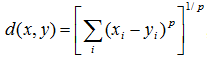 , when p = 1, Minkowsky distance is block distance, when p = 2, Minkowski distance is Euclidian distance.
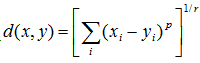 .
.

 method, B – Ward’s method")