Descriptive statistics can be grouped in 4 categories depending on their aim:
1) The estimation of central tendency of data,
2) The measures of variability,
3) The search for outliers,
4) The assessment of symmetry of data distribution.
Estimation of central tendency
For normally distributed data the mean (arithmetic average, usually designated as M or µ) is the typical value which is used in a report or journal article. However, this parameter is of limited value without estimation of the variability of the data. Therefore we should at least report three values – the mean, the standard error of the mean, and the sample size. Another variant is to report the mean and the standard deviation along with the sample size.
The median is another measure of central tendency and is usually reported when the data are not normally distributed. It indicates central value in a ranged dataset.
The mode is the most frequent value; it is a third measure of central tendency.
In the case of the median or mode it is better to give a range not by standard error or deviation but with interquartile range.
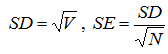
The measures of variability include the standard error (SE or m), the standard deviation (SD or σ), the variance (V) and the range. The first three measures are related in the following ways:
, where N – is the number of observations.
The standard deviation represents a measure of the degree to which individual observations in a dataset deviate from the mean value. In other words, it is an average deviation of all values from the mean. Standard deviation and 95% confidence interval are the best tests which should be used if the objective is to describe dataset itself.
The variance simply is the square of standard deviation.
The standard error of the mean together with 95% confidence interval should be used when the purpose is to assess maternal population rather than dataset itself. A 95% confidence interval provides a range of values within which the true population value of interest is likely to lie.
Very often a question arises in mind of researchers during description of a dataset – which measure of variability should be used, standard deviation or standard error of the mean? These statistics assess different things: standard deviation estimates the variability among individual observations in a dataset, while a standard error of the mean estimates the theoretical variability among means of samples derived from the same population. Many researches use standard error just for ‘cosmetic’ purpose because its value is smaller. However, accepted guidelines recommend using standard deviation because standard error provides no estimation of data variability (Kyrgidis and Triaridis, 2010). Standard errors should be reported only when the maternal population and not the sample is concerned.
Another measure often reported is the coefficient of variation. This measure provides a unitless measure of the variation of the data by translating it into a percentage of the mean value.
Search for outliers. Looking at the minimum and maximum values allows understanding if these values fall within expected range for these data. If a value is unexpectedly small or large, we should examine our original data to see whether some typing mistakes occur. If there are corrections that need to be made, they should be done before continuing. When some values are unexpectedly large are small, but are actual values, it may indicate that the data are not normally distributed. In that case we may consider using nonparametric procedures in further analyses. It may also indicate that the central tendency of data would be better described by median or mode rather than by mean value.
When many independent random factors act in an additive manner to create variability, the dataset on a histogram follows a bell-shaped distribution called the normal (or Gaussian distribution).
The normal distributions are a very important class of statistical distributions. All normal distributions are symmetric and have bell-shaped density curves with a single peak.
Figure adopted from here
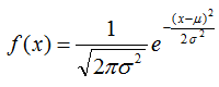
A normal distribution can be defined by two parameters, the mean and the standard deviation:
, where µ - the mean and σ – the standard deviation.
A measure that helps to decide normality is skewness and kurtosis. The skewness measure indicates the level of non-symmetry. If the distribution of the data is symmetric then skewness will be close to zero value. The farther it is from 0, the more skewed the data are. The kurtosis is a measure of the peakedness of the data. Similarly, for normally distributed data the kurtosis has zero value. As with skewness, if the value of kurtosis is too big or too small, there is a concern about the normality of the distribution.
There are general rules to recognize a normal and non-normal distribution:
1) In a perfect normal frequency distribution, the mean, median and mode are equal, and even if outliers are present the data are no bimodal or multimodal; they are continuous and symmetrically distributed around the central point.
2) In a perfect normal frequency distribution:
68% of samples fall between ± 1 standard deviations from the mean
95% of samples fall between ± 2 standard deviations from the mean
99.7% of samples fall between ± 3 standard deviations from the mean.
3) Statistical methods which determine whether one distribution (of experimental data) is significantly different from another (of hypothetical normally distributed data) can be used, such as Kolmogorov-Smirnov and Shapiro-Wilk tests.
4) Normal probability plots can be built, such as the probability-probability (P-P) and the quantile-quantile (Q-Q) plots. The Q-Q plot is more widely used, but both these plots refer to so-called probability plots and hence sometimes confusion is created. In general, deviances from the normality in the tails of the distribution are better detected by the Q-Q plot, whereas deviances near the mean of the distribution are better highlighted by the P-P plot.


 , where N – is the number of observations.
 , where µ - the mean and σ – the standard deviation.