The purpose of discriminant analysis is to predict value of categorical dependent variable based on values of predictors. To some extent it is similar to multiple linear regression, but outcome variable is categorical with 2 or more categories instead of continuous like in linear regression. Discriminant analysis includes several assumptions, such as predictor variables must be normally distributed, categories of outcome variable must be well-defined and mutually excluded, sizes of groups (categories) of dependent variables should be similar and should be at least five times the number of predictors.
Discriminant analysis produces several linear equations (discriminant functions), number of which corresponds the number of categories of dependent variable, or the number of categories minus one:
 ,
,
where D – discriminant function, v – the discriminant coefficient of weight of predictor variable, X – predictor variable, k – constant, i – the number of predictors.
Discriminant function is aimed to maximize distances between the categories. In general, there are two approaches in discriminant analysis. SPSS software produces number of discriminant functions equal to the number of categories of dependent variables minus one, and then membership of future cases is determined by closer location of its function to a mean value of present functions of categories. In some other statistical software (for example, in STATISTICA) the number of discriminant functions is equal to the number of categories and during predicting membership of new case, it is accepted to belong to that category for which the value of function is higher.
Selected examples on application of discriminant analysis in microbiological studies
|
Dependent variable
|
Predictor variables
|
Reference
|
|
Modes of action of antifungal compounds
|
Metabolic footprints of Saccharomyces cerevisiae
|
Allen et al., 2004
|
|
Sources of fecal contamination
|
Disk diffusion inhibition zones for different antimicrobials
|
Kaneene et al., 2007
|
|
In vitro antimalarial activity of new compounds against liver stages of Plasmodium
|
Topological indices of chemical compounds
|
Mahmoudi et al., 2008
|
|
Presence of systemic candidiasis
|
IgG responses against the antigens of Candida albicans
|
Clancy et al., 2008
|
|
Models of subacute ruminal acidosis induction in dairy cattle
|
Duration of rumen pH below 5.6, free rumen lipopolysaccharide, rumen microbial community dynamics, and serum haptoglobin
|
Khafipour et al., 2010
|
|
Spores samples of Bacillus cereus grown on different media
|
Cellular fatty acid methyl ester profiles
|
Ehrhardt et al., 2010
|
|
Intestinal bacterial community composition, prevalence of butyrate production pathway genes, and occurrence of Escherichia coli virulence factors in ileum-cannulated growing pigs
|
Nonstarch polysaccharides fractions
|
Metzler-Zebeli et al., 2010
|
|
Phage types of Salmonella enteritidis
|
Fourier transform infrared spectra
|
Preisner et al., 2010
|
|
Mycobacterium tuberculosis culture-positive sputum
|
Different electronic nose technology
|
Kolk et al., 2010
|
|
Animal source of Escherichia coli
|
Virulence factors
|
David et al., 2010
|
Performing discriminant analysis in SPSS
Let us discuss the following example.
We want to develop a model for prediction of presence of infection in peripancreatic fat tissue in patients with pancreonecrosis before operation, based on data of clinical and laboratory examination of a patient. The presence of microorganisms in peripancreatic fat (infectious pancreatits) is difficult to diagnose before operation because it is difficult to take sample and to do bacteriological examination before surgical opening of site of infection. However, early knowledge about infection may be useful in the choice of antibiotic treatment scheme.
In order to build prognosis model we retrospectively analyzed data of clinical-laboratory examination in 68 patients with pancreonecrosis on admission to hospital and compared the results of examination with post-operative diagnosis. Thus, the patients were divided into two groups – with sterile pancreonecrosis (21 patients) and with infectious pancreonecrosis (47 patients). We have selected only the variables in values of which there were significant differences between these two groups. Among different clinical and laboratory parameters only two appeared to have significant differences in sterile and infected patients – ratio between eosinophiles and lymphocytes in peripheral blood (ELR) and assessment of patient’s severity state by the Simplified Acute Physiology Score III (SAPS III) (Metnitz et al., 2005). Finally, we have produced the following dataset (see Example 8). Patients with sterile forms were designated as group “0” and with infective forms as group “1”.
Variables with significant differences in patients with sterile and infectious pancreonecrosis during admission to a hospital
|
N
|
Group of patients
|
ELR
|
SAPS III
|
|
1
|
0
|
0.000
|
51
|
|
2
|
0
|
0.167
|
51
|
|
3
|
1
|
0.083
|
47
|
|
4
|
0
|
0.100
|
36
|
|
5
|
0
|
0.091
|
44
|
|
6
|
1
|
0.077
|
55
|
|
7
|
1
|
0.077
|
49
|
|
8
|
1
|
0.133
|
58
|
|
9
|
1
|
0.400
|
54
|
|
10
|
1
|
0.000
|
47
|
|
11
|
0
|
0.091
|
43
|
|
12
|
1
|
0.000
|
49
|
|
13
|
1
|
0.162
|
47
|
|
14
|
1
|
0.067
|
62
|
|
15
|
1
|
0.000
|
47
|
|
16
|
1
|
0.400
|
47
|
|
17
|
1
|
0.000
|
57
|
|
18
|
1
|
0.059
|
51
|
|
19
|
0
|
0.167
|
33
|
|
20
|
1
|
0.167
|
45
|
|
21
|
1
|
0.000
|
41
|
|
22
|
1
|
0.000
|
47
|
|
23
|
1
|
0.154
|
47
|
|
24
|
1
|
0.000
|
47
|
|
25
|
1
|
0.111
|
60
|
|
26
|
0
|
0.000
|
53
|
|
27
|
1
|
0.063
|
51
|
|
28
|
1
|
0.000
|
53
|
|
29
|
0
|
0.074
|
42
|
|
30
|
1
|
0.000
|
51
|
|
31
|
1
|
0.000
|
50
|
|
32
|
0
|
0.121
|
42
|
|
33
|
1
|
0.017
|
60
|
|
34
|
1
|
0.000
|
51
|
|
35
|
0
|
0.400
|
47
|
|
36
|
1
|
0.071
|
42
|
|
37
|
1
|
0.000
|
55
|
|
38
|
0
|
0.042
|
42
|
|
39
|
0
|
0.000
|
50
|
|
40
|
1
|
0.000
|
57
|
|
41
|
0
|
0.029
|
42
|
|
42
|
0
|
0.273
|
52
|
|
43
|
1
|
0.000
|
60
|
|
44
|
1
|
0.000
|
51
|
|
45
|
0
|
0.250
|
50
|
|
46
|
1
|
0.200
|
42
|
|
47
|
0
|
0.091
|
50
|
|
48
|
1
|
0.029
|
54
|
|
49
|
1
|
0.024
|
42
|
|
50
|
1
|
0.000
|
53
|
|
51
|
0
|
0.100
|
49
|
|
52
|
1
|
0.125
|
42
|
|
53
|
1
|
0.250
|
55
|
|
54
|
1
|
0.000
|
42
|
|
55
|
1
|
0.056
|
47
|
|
56
|
0
|
0.000
|
53
|
|
57
|
1
|
0.000
|
42
|
|
58
|
0
|
0.333
|
60
|
|
59
|
1
|
0.000
|
63
|
|
60
|
1
|
0.000
|
63
|
|
61
|
1
|
0.125
|
55
|
|
62
|
0
|
0.063
|
42
|
|
63
|
0
|
0.111
|
33
|
|
64
|
1
|
0.000
|
60
|
|
65
|
1
|
0.000
|
55
|
|
66
|
1
|
0.000
|
49
|
|
67
|
1
|
0.028
|
56
|
|
68
|
1
|
0.294
|
56
|
To start discriminant analysis in SPSS:
1) Click the Analyze menu, point to Classify, and select Discriminant… :
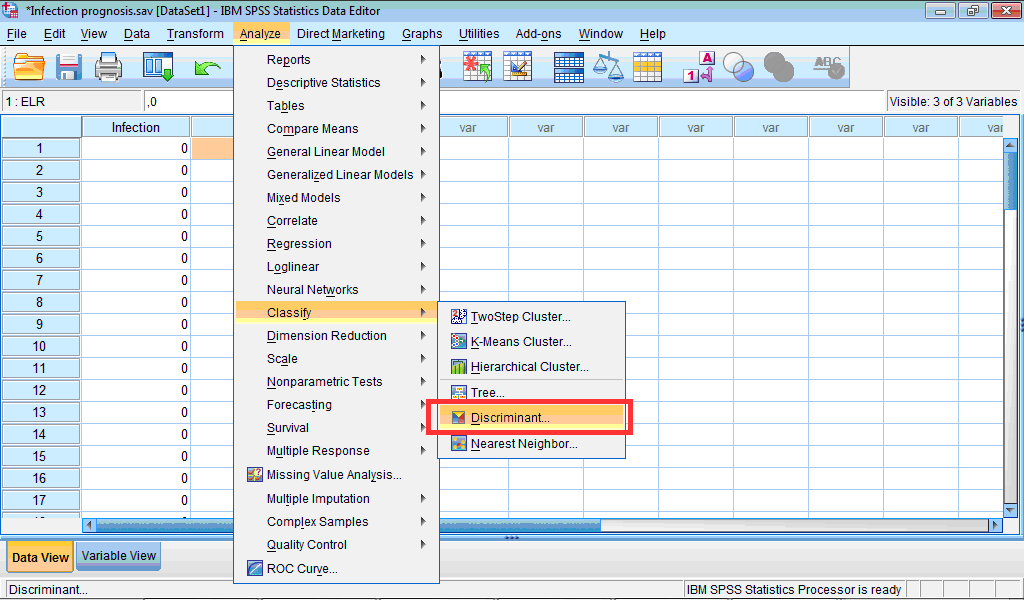
The Discriminant Analysis dialog box opens:
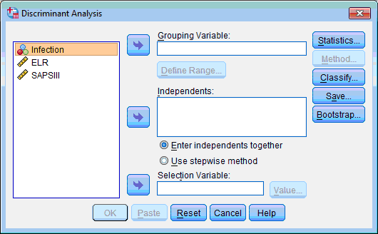
2) Select the grouping variable (“Infection”); click the upper transfer arrow button  . The selected variable is moved to the Grouping Variable: list box.
3) Click the Define Range… button. The Discriminant Analysis: Define dialog box opens:
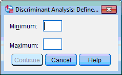
4) Enter the lowest and highest codes for the groups (in our example it is 0 and 1) in correspondent boxes. Click the Continue button, this returns you to the Discriminant Analysis dialog box.
5) Select the predictor variables (“ELR” and “SAPSIII”); click the next transfer arrow button  . The selected variables are moved to the Independents: list box.
6) By default Enter independents together method is selected, but if necessary Use stepwise method may be selected. Let us leave default settings.
7) Click the Statistics… button. The Discriminant Analysis: Statistics dialog box opens:
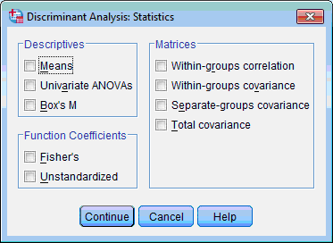
8) Select Means, Univariate ANOVAs, Box’s M, Unstandardized and Within-Groups Correlation check boxes. Click the Continue button, this returns you to the Discriminant Analysis dialog box.
9) Click the Classify… button. The Discriminant Analysis: Classification dialog box opens:
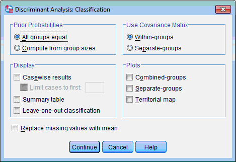
10) In the Prior Probabilities section select Compute from group sizes, in the Display section select Summary table and Leave-one-out classification, in the Use Covariance Matrix section leave selected by default Within-Groups, in the Plots section select all plots. Click the Continue button, this returns you to the Discriminant Analysis dialog box.
11) Click the Save button. The Discriminant Analysis: Save dialog box opens:
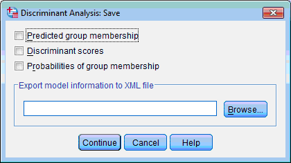
12) Select all check boxes and click the Continue button.
13) Click the OK button in the main dialog box. An Output Viewer window opens with results of discriminant analysis.
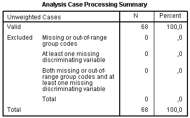
Results of discriminant analysis are displayed in a number of tables and figures. Like for every analysis, the table Analysis Case Processing Summary contains the information about cases included in the analysis:
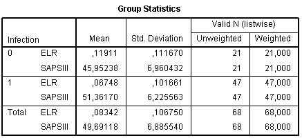
The next table is Group Statistics with means and standard deviations of the predictor variable in the every group of outcome variable. Look at this table gives rough preliminary information about differences between values of predictor variables between groups, however, without indicating statistical significance:
The Tests of Equality of Group Means provides further information about significance of differences between values of predictor variables in the groups. If there are no differences, it is not worthwhile to continue discriminant analysis. In our example significant differences present only in the variable “SAPS III”. However, significance of ELR is also close to 0.05, therefore, there may be a sense to keep this variable in the model and to compare results with and without it:

The
Pooled Within-Groups Matricestable evaluates intercorrelations between variables. In our example intercorrelation is very low (0.022) which support an idea about including both variables in the analysis:

In contrast to ANOVA, where basic assumption is the equality of variances for each group, in discriminant analysis basic assumption is the equality of variances-co-variances matrix. The null hypothesis states that matrix of covariances is equal between groups formed by the dependent variable. If the null hypothesis is proved and differences are not significant, it indicates desired result. Box’s M test is aimed to test this assumption.
The section Box’s Test of Equality of Covariance Matrices contains necessary data to assess equality of covariance matrices:
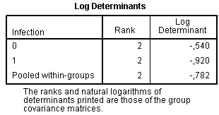
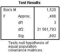
Significance level 0.692 indicates the desired result that the null hypothesis can be accepted. However, even when p level of M is significant (p<0.05) using large dataset, it is not regarded as very important drawback. If there are several compared groups and M is significant, then groups with very small absolute values of log determinants should be deleted and discriminant analysis repeated without them.
The next section of results is Summary of Canonical Discriminant Functions. It contains tables with eigenvalues and with Wilks’ Lambda:
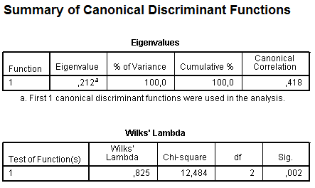
The table Eigenvalues provides information about produced discriminant functions. In SPSS number of discriminant functions is equal to number of groups minus one. We have only two groups (with sterile and infective pancreatitis) and because of this only one function (equation) is generated. The canonical correlation represents the multiple correlation between the predictors and the produced discriminant function. When there is only one function, canonical correlation is an index of overall model fit and it can be interpreted the same like R2 in linear regression as the proportion of variance explained. Our model explains very few variance: canonical correlation is 0.418, that is only 17.5% of total variance is explained by our model, and in future we should think how to improve the model.
Wilks’ Lambda to some extent is an opposite parameter to squared canonical correlation, it provides proportion of variance which is not explained by the model (82.5%). It also shows significance of the model (p = 0.002), therefore, in spite of poor describing total variance, significance of our model is still very high.
The next set of tables contains values of the discriminant model itself:
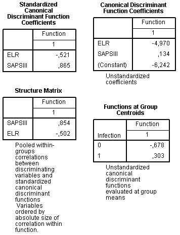
The Standardized Canonical Discriminant Function Coefficients table displays coefficients which indicate relative importance of each variable in the model. These coefficients have similar sense with beta coefficients of multiple regression. SAPS III is stronger predictor than ELR because its absolute value of standardized coefficient is higher. The sign indicates direction of the relationship: increase of SAPS III value enhances probability to fall into infective group, while for ELR relationship is opposite, high values are more favourable for a patient.
The Structure Matrix table shows the correlation of the variable with discriminant function and it is a one more way to assess importance of variables in the model. By many researchers it is considered as more accurate than the previous table and is preferred because of this. Results shown in the structure matrix are similar: SAPS III seems to be better predictor than ELR.
The table Canonical Discriminant Function Coefficients contains the unstandardized coefficients for the dicsriminant model, similar to B coefficient in the multiple regression. Therefore, our disrmininant function (D) can be written as:
 .
.
The next table is called Function at Group Centroids. Centroids are mean values of discriminant function for each group. This table is useful in supplementing the above-written equation, it gives information how to associate value of discriminant function with prognosis for each individual case. Cases with values near centroids are predicted to belong to that group, for example, patient with discriminant function -0.5 is predicted to belong to sterile group rather than to infected group. Cut-off may be defined as the difference between centroid values, that is “-0.375” (-0.678 – 0.303 = -0.375).
The Classification Statistics set of tables describes result of cases classification:
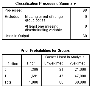
The Classification Processing Summary table summarizes processed and excluded cases. The Prior Probability for Groups table assesses probability of a case to fall into any of groups by chance accordingly to the ratio between sizes of groups. It indicates accuracy of prognosis by chance without using any models. For example, if we assign a random patient to an infected group, in 69.1% of cases this will be correctly.
Among results of discriminant analysis there are also two histograms called Canonical Discriminant Function with distribution of discriminant scores for each group. These charts help to assess how well groups are discriminated. When there is an overlap in distributions, the discriminant function is not very effective, like in our example:
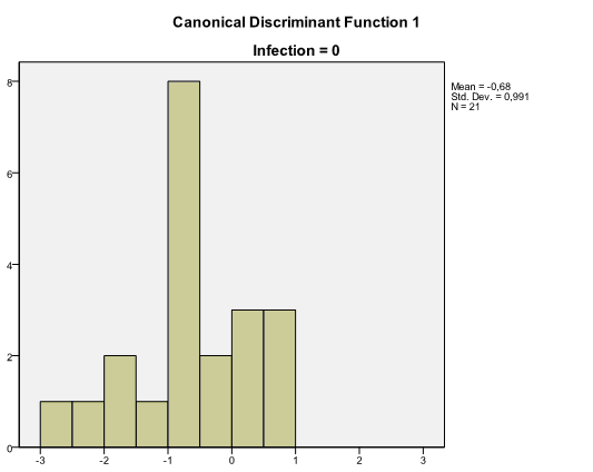
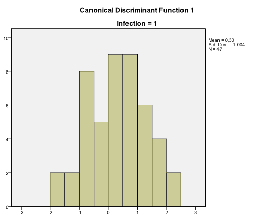
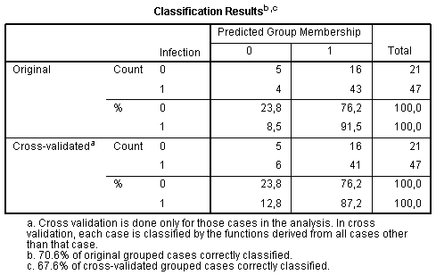
And, finally, the table Classification Results demonstrates whether classification of cases performed with built discrmininant model is successful. We can see that among infected patients 91.5% were classified correctly, while among sterile – only 23.8%:
During specification of parameters for discriminant analysis we selected to save additional variables, which now appeared in the Data Editor. The “Dis_1” variable contains group membership of each case, the “Dis1_1” variables has discriminant scores, the “Dis1_2” and the “Dis2_2” variables contain probability to belong to either first (sterile) or second (infected) group, respectively:
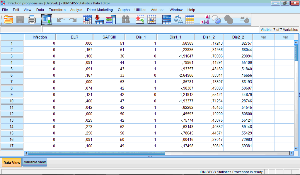
Information on which variable contains which data present in the labels of variables in the Variable View tab of the Data Editor.
Our discriminant model appears to be well in prognosis of presence of infected form, however, results for sterile forms were unsatisfactory, and, therefore, it is rational to try improving of the prognosis. We may try to add some additional variables or to apply another method of prognosis, for example logistic regression.
References
Allen J, Davey HM, Broadhurst D, Rowland JJ, Oliver SG, Kell DB. Discrimination of modes of action of antifungal substances by use of metabolic footprinting. Appl Environ Microbiol. 2004;70(10):6157-6165.
Kaneene JB, Miller R, Sayah R, Johnson YJ, Gilliland D, Gardiner JC. Considerations when using discriminant function analysis of antimicrobial resistance profiles to identify sources of fecal contamination of surface water in Michigan. Appl Environ Microbiol. 2007;73(9):2878-2890.
Mahmoudi N, Garcia-Domenech R, Galvez J, Farhati K, Franetich JF, Sauerwein R, Hannoun L, Derouin F, Danis M, Mazier D. New active drugs against liver stages of Plasmodium predicted by molecular topology. Antimicrob Agents Chemother. 2008;52(4):1215-1220.
Clancy CJ, Nguyen ML, Cheng S, Huang H, Fan G, Jaber RA, Wingard JR, Cline C, Nguyen MH. Immunoglobulin G responses to a panel of Candida albicans antigens as accurate and early markers for the presence of systemic candidiasis. J Clin Microbiol. 2008;46(5):1647-1654.
Khafipour E, Li S, Plaizier JC, Krause DO. Rumen microbiome composition determined using two nutritional models of subacute ruminal acidosis. Appl Environ Microbiol. 2009;75(22):7115-7124.
Ehrhardt CJ, Chu V, Brown T, Simmons TL, Swan BK, Bannan J, Robertson JM. Use of fatty acid methyl ester profiles for discrimination of Bacillus cereus T-strain spores grown on different media. Appl Environ Microbiol. 2010;76(6):1902-1912.
Metzler-Zebeli BU, Hooda S, Pieper R, Zijlstra RT, van Kessel AG, Mosenthin R, Gänzle MG. Nonstarch polysaccharides modulate bacterial microbiota, pathways for butyrate production, and abundance of pathogenic Escherichia coli in the pig gastrointestinal tract. Appl Environ Microbiol. 2010;76(11):3692-3701.
Preisner O, Guiomar R, Machado J, Menezes JC, Lopes JA. Application of Fourier transform infrared spectroscopy and chemometrics for differentiation of Salmonella enterica serovar Enteritidis phage types. Appl Environ Microbiol. 2010;76(11):3538-3544.
Kolk A, Hoelscher M, Maboko L, Jung J, Kuijper S, Cauchi M, Bessant C, van Beers S, Dutta R, Gibson T, Reither K. Electronic-nose technology using sputum samples in diagnosis of patients with tuberculosis. J Clin Microbiol. 2010;48(11):4235-4238.
David DE, Lynne AM, Han J, Foley SL. Evaluation of virulence factor profiling in the characterization of veterinary Escherichia coli isolates. Appl Environ Microbiol. 2010;76(22):7509-7513.
Metnitz PG, Moreno RP, Almeida E, Jordan B, Bauer P, Campos RA, Iapichino G, Edbrooke D, Capuzzo M, Le Gall JR; SAPS 3 Investigators. SAPS 3--From evaluation of the patient to evaluation of the intensive care unit. Part 1: Objectives, methods and cohort description. Intensive Care Med. 2005;31(10):1336-1344.

